Simulating Correlated Data
Thomas Ward April 26, 2021Summary
This article shows how to simulate correlated random variables, for any probability distributions, using the R programming language. No additional R packages beyond the functions found in base R will be needed.
In the example below I will generate three variables that are correlated with each other. Two are Poisson distributed count variables, while the other is a normally distributed continuous variable.
We will use the Gaussian copula to specify correlation between variables from different distributions in 3 steps:
- Generate a Normal(0, 1) distribution for each variable you wish to simulate, ensuring the desired correlation by sampling from a multivariate normal distribution.
- Perform the probability integral transform by applying the cumulative distribution function to each simulated variable that matches its probability distribution (in this case, Normal(0, 1)). This yields a uniform distribution from 0 to 1 for each variable. Each of these uniform distributions are still correlated with each other.
- Do inverse transform sampling to obtain variables distributed in their desired probability distributions (e.g., Poisson, Normal, Cauchy, etc.) by applying the appropriate quantile function (inverse cumulative distribution function).
Introduction
Simulating data is a crucial component of statistical modeling and helps you understand your model and data better (see Section 4 of Bayesian Workflow by Gelman et al. for more in-depth coverage).
I have recently been using multilevel models with varying slopes and intercepts and needed to simulate correlated data to ensure my models were working as expected. There are scattered resources on how to do so and different software packages that will automate the process, but I wanted to cement my understanding (and play around with a little linear algebra).
For this walkthrough, given that I’m a surgical resident, let’s simulate some variables for intra-operative surgical performance. We will generate four variables, three correlated, and one not. The variables will be as follows:
ak: the number of air knots (knots that are not tightened/secured all the way) a resident throws in a case. Given that it is a count variable, we will model it with the Poisson distribution.pp: the number of times a resident “passes point” (cuts/dissects farther than they should). This is a count variable, too, so it will also be modelled with the Poisson distribution.ptime: amount of time the resident spends practicing each week. This is a continuous quantity that we will model with a normal distribution.gs: the resident’s glove size. Glove sizes typically range from 5.5 to 9 in increments of 0.5, but for ease of modeling, we will make it a continuous variable, and model it with the Normal distribution. Glove size will not be correlated with the variables, as residents’ glove sizes, unless they are the wrong size, do not impact their performance.
Simulate the correlated predictors
We have three variables, ak, pp, and ptime that we need to
simulate together as they will be correlated. Remember, the correlation
of two variables can range from -1 to 1. We will simulate ak and pp
to have a positive correlation of 0.6, ak and ptime to have a
strongly negative correlation of -0.9, and pp and ptime to have a
moderately negative correlation of -0.5.
Sample from Multivariate Normal Distribution
First, we will take 10,000 samples for each variable from a multivariate normal distribution (MVNormal). Sampling from a MVNormal distribution is nice because we can specify how we want each variable to be correlated through it’s covariance matrix, Σ (Sigma). We will generate a Normal distribution with mean of 0 and standard deviation of 1 for each variable. Since the standard deviations of each distribution are 1, the covariance matrix is equivalent to the correlation matrix, which makes building the covariance matrix easy. Here is the Sigma for our distribution:
Sigma <- matrix(c(1, 0.6, -0.9, 0.6, 1, -0.5, -0.9, -0.5, 1), 3, 3)
Sigma

##      [,1] [,2] [,3]
## [1,]  1.0  0.6 -0.9
## [2,]  0.6  1.0 -0.5
## [3,] -0.9 -0.5  1.0
Now we will sample from the multivariate normal distribution,
MVNormal(0, Sigma). R does not have a MVNormal sampling function
built-in. You can either use the one in the MASS package, or use the
function below to replicate it with base R and some linear algebra:
mvrnorm <- function(n = 1, mu = 0, Sigma) {
  nvars <- nrow(Sigma)
  # nvars x n matrix of Normal(0, 1)
  nmls <- matrix(rnorm(n * nvars), nrow = nvars)
  # scale and correlate Normal(0, 1), "nmls", to Normal(0, Sigma) by matrix mult
  # with lower triangular of cholesky decomp of covariance matrix
  scaled_correlated_nmls <- t(chol(Sigma)) %*% nmls
  # shift to center around mus to get goal: Normal(mu, Sigma)
  samples <- mu + scaled_correlated_nmls
  # transpose so each variable is a column, not
  # a row, to match what MASS::mvrnorm() returns
  t(samples)
}
Now let’s generate the distributions for ak, pp, and ptime. I
named it APT to remind us which variable is in which column of the
returned matrix:
set.seed(1234)
APT <- mvrnorm(1e4, Sigma = Sigma)
You can see that the variables are correlated as we wanted:
cor(APT)

##            [,1]       [,2]       [,3]
## [1,]  1.0000000  0.5995270 -0.9012733
## [2,]  0.5995270  1.0000000 -0.5001539
## [3,] -0.9012733 -0.5001539  1.0000000

pairs(APT, labels = c("ak", "pp", "ptime"))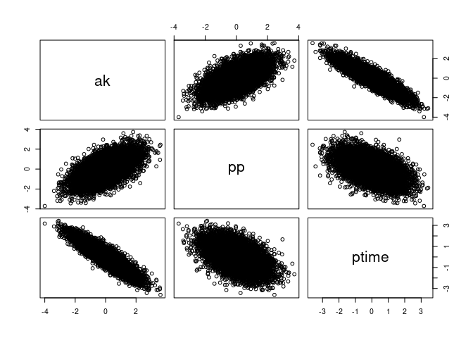
And that each is just a normal(0, 1) distribution. Take ak for
example:
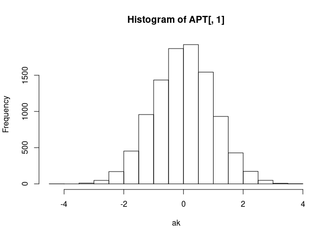
Probability integral transform
We now have three correlated Normal(0, 1) distributions. We can apply the cumulative distribution function (CDF) to each variable that matches the probability distribution that generated them to yield a uniform distribution from 0 to 1 for each variable. After this transformation, these uniform distributions will still be correlated! This is known as the probability integral transform.
We know the probability distribution that generated them is Normal(0,
1), so we can use the pnorm() function in R to apply the CDF for the
normal distribution and make the uniform distributions, U (a matrix
with one column for each variable):
U <- pnorm(APT, mean = 0, sd = 1)Let us take a look at the U for A (column 1):
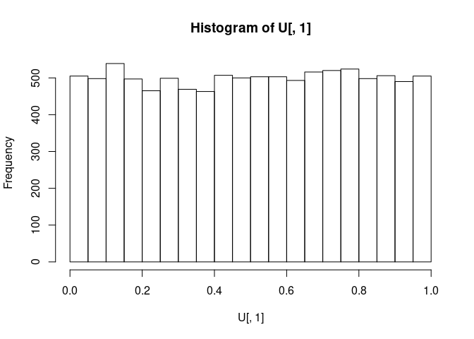
As expected, it is a uniform distribution from 0 to 1.
As we see below, these are still correlated, just like we wanted!
cor(U)

##            [,1]       [,2]       [,3]
## [1,]  1.0000000  0.5785758 -0.8935338
## [2,]  0.5785758  1.0000000 -0.4800510
## [3,] -0.8935338 -0.4800510  1.0000000

pairs(U, labels = c("ak", "pp", "ptime"))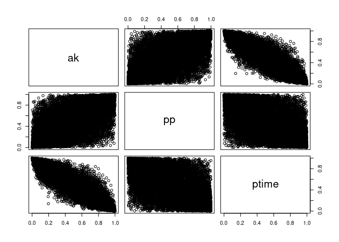
Inverse transform sampling
Now that we have correlated uniform distributions for each variable, we can do inverse transform sampling by applying the quantile function for the desired probability distributions.
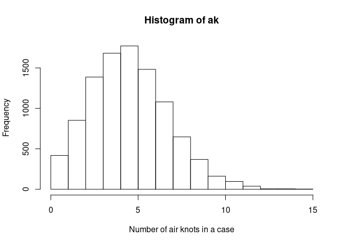
Air knot variable, ak
Our air knot variable, ak is in the first column of U. We will make
it a Poisson distribution with an average number of air knots of 5 per
case.
We can transform the first column of U, U[, 1], to match that
distribution with the qpois() function:
ak <- qpois(U[, 1], 5)Take a look at the distribution we made:
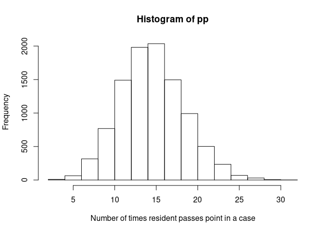
Passes point variable, pp
Our passes point variable, pp is in the second column of U. We will
make it a Poisson distribution with a mean of 15 “passing point”
happening per case. Again, we will use the quantile function for the
Poisson distribution, qpois(), this time on the second column of U,
U[, 2]:
pp <- qpois(U[, 2], 15)Take a look at the distribution we made:
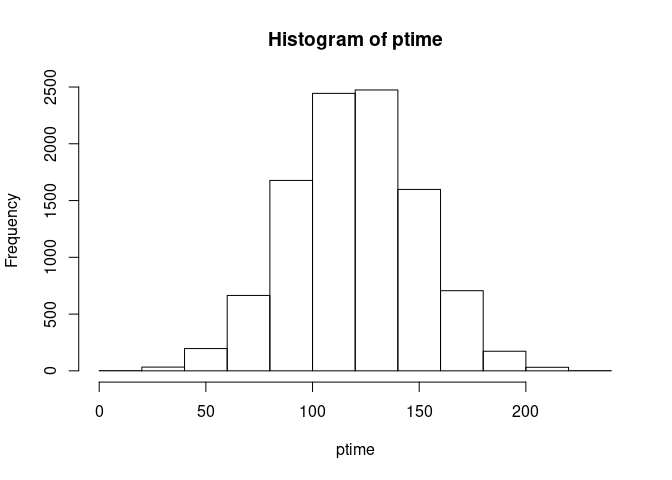
Practice time, ptime
Our practice time variable, ptime, is in the third column of U. It
represents the amount of time, in minutes, the resident spent practicing
that week. We will make it a Normal distribution with a mean of 120 and
standard deviation of 30.
Since we want a Normal distribution, we will use the quantile function
qnorm() on the third column of U, U[, 3]:
ptime <- qnorm(U[, 3], 120, 30)Take a look at the distribution we made:
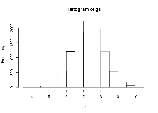
Sample non-correlated variable, glove size, gs
We do not need to sample this with MVNorm since it is not correlated to our other variables. We know sizes are between 5.5 and 9 and likely follow a normalish distribution that is centered around the midway point of 5.5 and 9 (7.25) with only a few outliers:
gs <- rnorm(1e4, 7.25, 0.875)Which looks like:
Inspection of variables generated
Now, after all the variable manipulation, did our original desired correlations hold up?
To remind ourselves, we wanted:
akandppto have a correlation of 0.6,
cor(ak, pp)

## [1] 0.5896031akandptimehave a correlation of -0.9,
cor(ak, ptime)

## [1] -0.8881121ppandptimehave a correlation of -0.5.
cor(pp, ptime)

## [1] -0.497877gsto be not correlated with any of the above.
cor(gs, ak)

## [1] 0.001217374cor(gs, pp)
## [1] 0.005355465cor(gs, ptime)
## [1] 0.001196094Perfect, everything simulated and kept the desired correlations!
We can visualize their correlations with pairs():
pairs(data.frame(ak, pp, ptime, gs))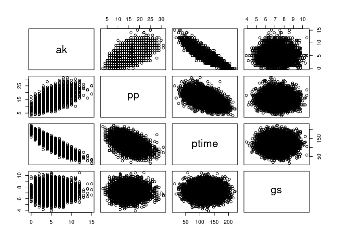
Now we are set to experiment with this simulated data.
Closing comments
Simulating correlated variables takes three straightforward steps:
- Sample correlated N(0, 1) distributions from a multivariate normal distribution.
- Transform them to correlated Uniform(0, 1) distributions with the normal CDF.
- Transform them to any correlated probability distribution you desire with that probability distribution’s inverse CDF.
I will caution that some distributions are harder to make correlate due to their nature, such as the log normal distributions and Bernoulli distributions. For log-normal distributions, I recommend simulating a normal distribution of the “logged” version of the variable to correlate the variables appropriately then exponentiating the result. While the exponentiated results will not correlate, you should be log-transforming the variable prior to modeling anyways, so log(variable) will still correlate.
I hope this article helps! Enjoy simulating complex relationships in data and seeing if your statistical models work and can recover their parameters. Please contact me with any questions or input on the article using any of the methods on my contact page.